Padded-CSR
A sparse storage format for dynamic sparse training on CPU
- 1. Why Sparse Matters
- 1.1 The Lottery Ticket
- 1.2 The Brain Runs on 20 Watts
- 1.3 So Why Did Dense Win?
- 1.4 Mask-on-Dense
- 1.5 The Gap SparseLab Targets
- 2. What Sparsity Actually Means
- 2.1 A Definition and a Picture
- 2.2 The Layer We'll Keep Using
- 3. Why Sparse Compute Is Hard
- 3.1 The First Naive Try: COO
- 3.2 The Insight: A Row Pointer
- 4. CSR, and Where It Breaks
- 4.1 CSR Stated Precisely
- 4.2 The Insertion Problem
- 4.3 Why DST Cares
- 5. Padded-CSR: The Fix
- 5.1 Building the Format
- 5.2 Per-Row Padding
- 5.3 Worked Example
- 5.4 Memory Accounting
- 6. The SpMM Kernel
- 6.1 What SpMM Computes
- 6.1b What SIMD Is
- 6.2 NEON SIMD + 2× Unroll
- 6.3 OpenMP Parallelism
- 7. The Backward Pass
- 7.1 Two Gradients
- 7.2 Cached Transpose
- 8. What We Got and What's Next
- 8.1 What v0.1 Ships
- 8.2 Try It
- 8.3 What's Next
- 8.4 Contribute
- 9. What Ideal Sparse Hardware Would Look Like
- 9.1 What GPUs Do (and Don't)
- 9.2 Where Sparse Accelerators Exist
- 9.3 The Ideal Sparse Chip
- 9.4 Why This Hasn't Happened Yet
SparseLab is a PyTorch library for training actually-sparse neural networks on CPU. This post is the long version — why sparse training matters, why it's been stuck behind a software and hardware gap for years, how a storage format called Padded-CSR breaks one piece of that gap open, and what the kernel that makes it fast actually looks like. No prior experience with sparse formats assumed.
1. Why Sparse Matters
1.1 The Lottery Ticket
In 2018, Jonathan Frankle and Michael Carbin at MIT published a paper called The Lottery Ticket Hypothesis. Their claim: inside every large, densely-connected neural network you train from random initialization, there's a much smaller subnetwork that — if you'd known which weights it was and trained only those from the start — would have reached the same accuracy with a fraction of the parameters.
They called these subnetworks winning tickets. The mental picture: training a big dense network is like buying a huge pile of lottery tickets so that at least one of them wins. Almost all the tickets are worthless. But you don't know which ones ahead of time, so you buy them all.
The experimental procedure was direct. Take a trained network. Prune the smallest-magnitude weights (set them to zero). Reset the remaining weights to their original random initialization. Train again from scratch, with the pruned weights held at zero. Result: you can reach the same accuracy at 10–20% of the parameters, sometimes less.
That was the crack in the floor. If 80–90% of a network's weights are deadweight, then training them is wasted compute, storing them is wasted memory, and multiplying by them at inference is wasted energy. A 70B-parameter model that's actually a 10B-parameter model in disguise is a dramatic thing.
1.2 The Brain Runs on 20 Watts
There's a biological version of the same argument. Your brain has roughly 86 billion neurons connected by ~100 trillion synapses. On any given moment, a vanishing fraction of them are active. Brains are extraordinarily sparse, both in connectivity (each neuron touches maybe 10,000 others, not all 86 billion) and in activity (most neurons are quiet most of the time).
And the whole organ runs on about 20 watts. A dim light bulb.
The GPUs approximating a fraction of what the brain does pull kilowatts each, scaled into datacenters that draw gigawatts. That gap between 20 watts and a gigawatt is not entirely fundamental — a lot of it is that we built silicon for the wrong workload.
1.3 So Why Did Dense Win?
If the lottery ticket hypothesis was already known in 2018 and brains have been doing sparse forever, why is basically every neural network in production today trained as a dense matrix multiplication?
The answer is hardware, and the hardware story has three layers.
Dense matmul is perfectly regular. A matrix multiplication C = A @ B where A is M×K and B is K×N does exactly M×N×K multiply-adds, in a predictable, cache-friendly pattern. Every row of A touches every column of B. Memory access is contiguous. Loop bounds are known at compile time. GPU vendors can build silicon that assumes this structure and pipeline the hell out of it — tensor cores, warp scheduling, coalesced memory access, the whole stack. An NVIDIA H100 SXM5 hits roughly 1,000 TFLOPS of dense FP16 tensor throughput (~500 TFLOPS on the PCIe variant).
Sparse matmul is the opposite of regular. If half the entries of A are zero and they're scattered around arbitrarily, the kernel has to chase pointers to find the live entries, emit indirect memory loads to fetch the right column of B, and tolerate unbalanced work across rows (some rows have many live entries, others have few). That's everything modern GPUs are bad at.
So the industry compromised. NVIDIA's Ampere generation introduced 2:4 structured sparsity: out of every four consecutive weights, exactly two must be zero. That's regular enough that tensor cores can accelerate it. But it caps sparsity at exactly 50%, and in practice the speedup is often modest — a 2024 analysis found the real gains often under 1.3×. Anything above 50% sparsity on a GPU falls back to dense matmul with zeros in the middle.
1.4 Mask-on-Dense: The Compromise That Kills the Memory Win
Faced with hardware that only likes dense math, the sparse-training research community did the obvious thing: simulate sparsity on top of dense hardware. Most sparse-training papers — Lottery Ticket, RigL, SET, SNIP, and many others — store the weight matrix as a regular dense tensor and keep a parallel binary mask that says which entries are "live."
MASK-ON-DENSE:
══════════════
  W      (dense, shape [512, 784], 4 bytes each)   = 1568 KB
  mask   (binary, shape [512, 784], 1 byte each)   =  392 KB
  Forward:  Y = (W * mask) @ X     # element-wise multiply first
  Backward: dW = dY @ Xᵀ           # full dense gradient
            dW *= mask             # zero out the dead entries

Compute: full dense matmul cost. Mask is "applied," not "skipped."
Memory: larger than pure dense, because we carry both W and mask.
This gives you the research artifact — you can run sparse-training algorithms, measure accuracy, publish results. It delivers no memory savings, because every zero is still stored. It delivers no compute savings, because the GPU still multiplies by the zeros (and then discards them). The only thing the mask saves is the conceptual cleanliness of saying "this weight is gone" — not the resources it consumes.
It's a paradigm that lets sparse-training research exist while quietly admitting that the hardware it runs on can't actually benefit from sparsity. That's not nothing — the algorithmic work has been real — but anyone who's tried to turn a mask-on-dense research paper into a production memory saving has hit this wall.
1.5 The Gap SparseLab Targets
This leaves an odd hole. We have:
- A theoretical reason to believe sparse networks work (lottery ticket, biology).
- A decade of algorithmic progress on how to find the live weights (RigL, SET, magnitude pruning, gradient-based criteria).
- Hardware that fundamentally doesn't want to run them at anything above 50% sparsity.
- A software ecosystem where "sparse training" means "dense training with a mask" — which gives up the whole point.
A researcher who wants to experiment with actual-sparse training — real sparse storage, real sparse kernels, real memory savings — doesn't have a place to do it. GPU vendors don't ship unstructured sparse training kernels. PyTorch's torch.sparse doesn't support training well. The wafer-scale chips that do accelerate unstructured sparsity (Cerebras) cost millions and aren't installable.
SparseLab's bet. The algorithmic case for sparse has been made — the lottery ticket, the biology, a decade of DST work. What's missing is the substrate: GPUs love dense, "sparse" in practice means mask-on-dense, and mask-on-dense gives up the memory savings that were the whole point. The software stack has to exist first, before hardware can optimize for it. If you can train a meaningful sparse network on a MacBook — real sparse storage, real kernels, real memory savings — then sparse-training research has a platform, and future sparse accelerators have a target. That's v0.1.
The rest of this post is about the technical substrate that makes actually-sparse training possible: how you represent a sparse matrix so that it's small in memory and fast to multiply and cheap to mutate during training. The format is called Padded-CSR. To motivate it, we need to first define what sparsity actually is, and why doing it properly is hard.
2. What Sparsity Actually Means
2.1 A Definition and a Picture
A sparse matrix is a matrix where most of the entries are exactly zero. "Most" isn't precisely defined — 50% is the rule of thumb where specialized storage formats start to win over plain dense storage, but in neural networks we typically care about 80% sparsity and up.
The standard quantities:
- nnz (“number of non-zeros”): how many entries are live. For an M×N matrix,
nnzis at mostM × N. - density:
nnz / (M × N). The fraction of the matrix that's live. - sparsity:
1 - density. The fraction that's zero.
A 90%-sparse 1000×1000 matrix has density = 0.1 and nnz = 100,000, which is 10% of the total 1,000,000 entries.
2.2 The Layer We'll Keep Coming Back To
Pick a concrete layer: the first linear of a tiny MNIST classifier. 784 inputs (the flattened 28×28 pixels), 512 hidden units. The weights are a 512×784 matrix (PyTorch stores nn.Linear weights as [out_features, in_features]):
LAYER: nn.Linear(784, 512)
══════════════════════════
Shape:              W ∈ ℝ^(512 × 784)
Total entries:      512 × 784       = 401,408
Dense memory (f32): 401,408 × 4 B   ≈ 1,568 KB ≈ 1.6 MB
Now suppose this layer has been trained with a sparse algorithm and 90% of its weights have been driven to exactly zero. Not “small,” literally zero. That leaves roughly 40,000 live entries, scattered more or less arbitrarily across the 512 rows.
WHAT THE TRAINED MATRIX LOOKS LIKE (schematic):
═══════════════════════════════════════════════
                (784 columns)
            ┌─────────────────────────┐
  Row 0:    │ .  .  .  X  .  .  . X . │  ← ~80 live entries
  Row 1:    │ .  X  .  .  .  .  . . . │  ← ~80 live entries
  Row 2:    │ .  .  .  .  .  .  . . . │  ← 0 live entries
  ...                                       ...
  Row 511:  │ X  .  X  .  .  .  . . . │  ← ~80 live entries
            └─────────────────────────┘
  (X = live nonzero,  . = exactly zero)

  nnz        ≈ 40,000
  density    ≈ 0.10
  sparsity   ≈ 0.90
Two things are true about this matrix, and they're what makes sparse hard.
First, storing it in dense format wastes 90% of the memory. 1.6 MB of RAM is holding ~360,000 values we know are zero. For a single MNIST layer that's fine. For a 70-billion-parameter language model, "90% of memory is zeros" is the difference between fitting on a GPU and not.
Second, multiplying it in dense format wastes 90% of the compute. A standard matrix-vector multiply performs M × N multiply-add operations. 90% of those operations are anything × 0 = 0. The hardware dutifully computes them anyway, because it has no way to know they're zero without checking each one — and checking would be slower than just multiplying.
3. Why Sparse Compute Is Hard
The goal is a storage format that satisfies three things at once: small memory footprint, fast matrix multiplication, and (for training) cheap mutation. Let's try to build one from scratch.
3.1 The First Naive Try: COO
The simplest sparse format is the coordinate list, or COO. For every live entry, store three things: its row, its column, and its value. Skip the zeros entirely.
COORDINATE LIST (COO):
══════════════════════
Dense 4×6 matrix (we'll use this toy for the rest of the section):
  [ 0  0  3  0  0  0 ]
  [ 0  0  0  0  0  0 ]
  [ 2  0  0  0  5  0 ]
  [ 0  7  0  0  0  4 ]

  nnz = 5 (five live entries)

COO encoding (three parallel arrays, one entry per live value):
  rows    = [ 0, 2, 2, 3, 3 ]
  cols    = [ 2, 0, 4, 1, 5 ]
  values  = [ 3, 2, 5, 7, 4 ]

Storage: 3 integers/floats per live entry × 5 entries = 15 items.
Dense:   24 items. Modest win on this toy, large at real scale.
This solves the memory problem. For a 90%-sparse matrix, COO uses roughly 30% of dense storage (three numbers per live entry instead of one per total entry, at the same int32/float32 width).
But it fails the multiplication test. Computing y = W x means, for each output row i, summing W[i, j] × x[j] over all columns j where W[i, j] is live. With COO, to find row i's live entries we have to scan the entire rows array looking for places where rows[k] == i:
COMPUTING y = W x WITH COO:
═══════════════════════════
for i in 0..nrows:
    y[i] = 0
    for k in 0..nnz:
        if rows[k] == i:               # ← most of the time, false
            y[i] += values[k] × x[cols[k]]

Total work: O(nrows × nnz).

For our 512 × 784 MNIST layer at 90% sparsity:
  nrows × nnz = 512 × 40,000 ≈ 20 million inner-loop iterations.
  The if condition is false ~98% of the time.

Branch predictor is upset. The cache hates it. This is slow.
We could sort the entries by row so the if at least stops early, but we'd still scan past every other row's entries. What we really want is to jump directly to row i's entries in constant time.
3.2 The Insight: A Row Pointer
Sort the entries by row. Then build a small side-table that records, for each row, the index where its entries begin in the sorted list. Looking up a row is now a single array read instead of a linear scan.
SORTED COO + ROW POINTER:
═════════════════════════
Same matrix. Entries sorted by (row, then col):

  rows    = [ 0, 2, 2, 3, 3 ]    ← already sorted by row
  cols    = [ 2, 0, 4, 1, 5 ]
  values  = [ 3, 2, 5, 7, 4 ]

Build a row pointer: row_start[i] = index into `values` where
row i's entries begin.

  row_start = [ 0, 1, 1, 3, 5 ]
               ↑  ↑  ↑  ↑  ↑
               │  │  │  │  └── end of array (= nnz = 5)
               │  │  │  └───── row 3 starts at index 3
               │  │  └──────── row 2 starts at index 1
               │  └─────────── row 1 starts at index 1 (empty: start = end)
               └────────────── row 0 starts at index 0

Row i's entries are indices [row_start[i], row_start[i+1]).
Row 0: slice [0, 1)  = values[0..0]  = [3]
Row 1: slice [1, 1)  = empty
Row 2: slice [1, 3)  = values[1..2]  = [2, 5]
Row 3: slice [3, 5)  = values[3..4]  = [7, 4]
Two observations:
First, row_start has length nrows + 1. The extra entry at the end lets us always write row_start[i+1] without going out of bounds, which means every row — including the last — has a well-defined "end" we can subtract from its "start."
Second, once we have row_start, we don't need the rows array at all. It contained exactly the information we just compressed into row_start, only verbosely. Drop it.
That's CSR: Compressed Sparse Row. Three arrays — values, col_indices (the old cols), and row_ptr (the row_start we just built).
4. CSR, and Where It Breaks
4.1 CSR Stated Precisely
We just derived CSR. Let's pin down the format and confirm it fixes the multiplication problem:
STANDARD CSR FORMAT:
════════════════════
values[]        — length nnz. The live values, stored row-by-row,
                  sorted by column within each row.

col_indices[]   — length nnz. For each value, which column it's in.

row_ptr[]       — length nrows+1. row_ptr[i] is the index into
                  values[] where row i begins. row_ptr[i+1] is
                  where row i ends (exclusive).

Row i's live entries:  values[row_ptr[i] : row_ptr[i+1]]
Their columns:         col_indices[row_ptr[i] : row_ptr[i+1]]
Applied to the same 4×6 example:
CSR ENCODING (same 4×6 matrix):
═══════════════════════════════
  values      = [ 3, 2, 5, 7, 4 ]      (5 floats)
  col_indices = [ 2, 0, 4, 1, 5 ]      (5 ints)
  row_ptr     = [ 0, 1, 1, 3, 5 ]      (nrows+1 = 5 ints)

  Storage: 5 + 5 + 5 = 15 items vs 24 dense items.

Break-even point: for float32 values and int32 column indices,
CSR becomes smaller than dense at about 50% sparsity. At 90%
sparsity (the regime we care about), CSR uses roughly 20% of
dense storage.
And the multiplication kernel is now trivial:
COMPUTING y = W x WITH CSR:
═══════════════════════════
for i in 0..nrows:
    y[i] = 0
    for k in row_ptr[i] .. row_ptr[i+1]:   # just this row's entries
        y[i] += values[k] × x[col_indices[k]]

Total work: O(nnz). No wasted iterations.

For the 512 × 784 MNIST layer at 90% sparsity:
  COO version:   ~20 million inner iterations
  CSR version:       40,000 inner iterations
  ~500× fewer loop bodies executed.
CSR is not new. It dates to the 1960s and it's the foundational format for scientific sparse computing. PyTorch has torch.sparse_csr_tensor. SciPy has scipy.sparse.csr_matrix. Every serious CPU and GPU numerical library ships a CSR matrix-multiplication kernel. For static sparse matrices — sparse matrices whose pattern of live entries doesn't change — CSR is basically done.
Training, unfortunately, doesn't have static sparse matrices.
4.2 The Insertion Problem
CSR stores live entries contiguously in values[] and col_indices[]. That's what makes the SpMM kernel fast — the inner loop walks contiguous memory. But contiguity has a cost: you can't insert a new entry anywhere without shifting everything after it.
Say we want to add a live entry at (row 2, col 2) with value 6 in our example:
INSERTING (2, 2, 6) INTO CSR:
═════════════════════════════
Before:
  values      = [ 3, 2, 5, 7, 4 ]
  col_indices = [ 2, 0, 4, 1, 5 ]
  row_ptr     = [ 0, 1, 1, 3, 5 ]

Row 2's entries are values[1..3] = [2, 5]. The new entry (col=2)
must be inserted between col=0 and col=4 to keep the row sorted.

Step 1: Allocate new arrays of length nnz+1 = 6.
Step 2: Copy all entries before the insertion point unchanged.
Step 3: Write the new entry.
Step 4: Copy all entries after the insertion point, SHIFTED BY 1.
Step 5: Increment row_ptr[3] and row_ptr[4] (every row after
        the insertion point is now offset by +1).

After:
  values      = [ 3, 2, 6, 5, 7, 4 ]   ← 5, 7, 4 all shifted right
  col_indices = [ 2, 0, 2, 4, 1, 5 ]   ← same
  row_ptr     = [ 0, 1, 1, 4, 6 ]      ← rows 3+ bumped by 1

Cost: copy everything after the insertion point.
      Worst case (insert at row 0): O(nnz).
      Average case: O(nnz / 2).
One insertion costs O(nnz) work. For a 90%-sparse 10M-parameter transformer layer, that's ~1M live entries to shift per insertion. Do a thousand insertions per topology update, and you're copying gigabytes of memory every few hundred training steps.
4.3 Why DST Cares
Dynamic Sparse Training (DST) is the family of algorithms where the sparsity pattern changes during training. RigL, SET, and their descendants periodically drop the least useful weights and grow new ones in their place. The specific schedules vary, but the pattern is consistent: every N steps (typically 100-1000), drop some fraction of the live entries and add the same number of new ones elsewhere.
TYPICAL DST UPDATE (e.g., RigL on a 1M-live-entry layer):
═════════════════════════════════════════════════════════
Every 100 training steps:
  1. Drop 10% of live entries (100,000 entries removed)
  2. Grow 10% new entries at high-gradient locations

Per update, using standard CSR:
  Drops: 100,000 × O(nnz) shifts ≈ 10¹¹ operations
  Grows: 100,000 × O(nnz) shifts ≈ 10¹¹ operations
  Total: ~2 × 10¹¹ memory operations, about 2 seconds of pure
  copying on modern hardware.

Per update, using dense-mask simulation:
  Drops/grows: O(live_entries) bit operations — ~microseconds.
  But: the entire dense weight matrix (10M floats = 40MB) stays
  allocated. No memory win.

Per update, using Padded-CSR:
  Drops: in-place, set col=-1, val=0. O(1) per drop.
  Grows: in-place, fill next padding slot. O(1) per grow,
  amortized over occasional row-resize.
  Total: microseconds.
This is the fundamental tension. CSR gives us real sparse storage but bad mutation performance. Dense-mask simulation gives us fast mutation but no memory win. We want both — real sparse storage AND fast mutation. Hence Padded-CSR.
The problem in one line. CSR is great until the sparsity pattern changes — every topology mutation is O(nnz), and DST mutates topology every few hundred steps. We need a format that's structurally like CSR but allows O(1) insertions.
5. Padded-CSR: The Fix
The idea: reserve extra capacity per row, so most insertions land in an already-allocated slot and only bump a counter.
5.1 Building the Format, One Array at a Time
Let's start from CSR and add only what we need, one piece at a time. CSR has three arrays: values, col_indices, and row_ptr. What breaks when we try to add padding?
Step 1: Make the slot arrays longer. In CSR, values[] and col_indices[] have exactly nnz entries — one per live value, packed tight. To add padding, we make these arrays longer. Each row gets some extra slots beyond its current live count. The arrays now have length total_capacity (the sum of all rows' capacities), not nnz.
ARRAY 1: values[]       (length = total_capacity)
  Live slots hold real weight values.
  Padding slots hold 0.0f.

ARRAY 2: col_indices[]  (length = total_capacity)
  Live slots hold the column index (0 ≤ col < ncols).
  Padding slots hold -1 (a sentinel that says "this slot is empty").
These two are the same as CSR, just with gaps. The kernel skips padding slots by checking col_indices[k] != -1, or (better) by knowing how many live entries each row has. Which brings us to the next problem.
Step 2: Split row_ptr into row_start. CSR's row_ptr encodes both "where does row i start?" and "where does row i end?" in a single array (the end of row i is row_ptr[i+1]). That works because rows are packed tight — row i ends exactly where row i+1 begins.
With padding, that's no longer true. Row i's live entries end before its padding, and the padding ends before row i+1's live entries start. We need to know where each row's region begins independently.
ARRAY 3: row_start[]    (length = nrows)
  row_start[i] = index into values[]/col_indices[] where row i's
  allocated region begins (both live entries and padding).
Step 3: Track how many entries are actually live. We know where row i starts (row_start[i]), but we need to know how many of those slots are live vs padding. Without this, the kernel would have to scan for col_indices == -1 sentinels to find the boundary — slow and branch-heavy.
ARRAY 4: row_nnz[]      (length = nrows)
  row_nnz[i] = number of LIVE entries in row i.
  Within row i's region, slots [row_start[i], row_start[i] + row_nnz[i])
  are live. Everything after that is padding.
This is the key invariant: live entries come first, padding comes after. The SpMM kernel loops from row_start[i] to row_start[i] + row_nnz[i] and never touches padding. Inserting a new entry means writing to slot row_start[i] + row_nnz[i] (the first padding slot) and incrementing the counter. O(1).
Step 4: Track how much capacity each row has. When we insert, we need to know if there's still padding left. If row_nnz[i] == row_capacity[i], the row is full and we need to resize (allocate more slots, copy the row, update pointers). Without tracking capacity, we'd have to compute it from row_start[i+1] - row_start[i], which only works if rows are laid out contiguously — and after a resize, they might not be.
ARRAY 5: row_capacity[] (length = nrows)
  row_capacity[i] = total allocated slots for row i (live + padding).
  Always: row_capacity[i] ≥ row_nnz[i].
Step 5: A version counter for cache invalidation. The backward pass needs the transpose of W (Section 7.2). Computing a transpose is expensive, so we cache it. But when the topology changes (entries added or removed), the cached transpose is stale. Rather than hashing the whole structure to detect changes, we keep a single counter that bumps on every structural mutation.
ARRAY 6: topology_version  (single int64)
  Monotonically increasing counter. Bumps on every structural
  mutation (insert, delete, row resize). Downstream caches
  (like the transpose cache in Section 7.2) compare their
  stored version against this to decide whether to rebuild.
That's the full format. Six arrays, each motivated by a specific need:
PADDED-CSR SUMMARY:
═══════════════════
  values[]         — the weights (same as CSR, but with padding gaps)
  col_indices[]    — which column each weight belongs to (-1 = padding)
  row_start[]      — where each row's region begins
  row_nnz[]        — how many entries in each row are live
  row_capacity[]   — how many total slots each row has
  topology_version — cache-invalidation counter
5.2 Per-Row Padding
How much padding per row? SparseLab's default is 20% (padding_ratio = 0.2). The formula:
row_capacity[i] = max(1, ceil(row_nnz[i] × (1 + padding_ratio)))

Examples (padding_ratio = 0.2):
  row_nnz = 0  → capacity = 1    (floor at 1, so empty rows can
                                   accept at least one insertion)
  row_nnz = 5  → capacity = 6    (ceil(5 × 1.2) = 6)
  row_nnz = 100 → capacity = 120 (ceil(100 × 1.2) = 120)
  row_nnz = 1000 → capacity = 1200
Why 20%? RigL and SET drop/grow roughly 10% of live entries per update. A 20% padding buffer means most grows hit existing capacity without triggering a row resize. Empirically, a 90%-sparse layer trained with RigL on a 100-step schedule needs a row resize ~once every 50-100 updates.
The floor-at-1 rule matters for a subtle reason: rows that start empty (row_nnz = 0) would otherwise get capacity = 0, and any grow attempt would trigger an expensive resize. Reserving one slot for empty rows keeps the O(1) path available for the first entry.
5.3 Worked Example
Let's take the same 4×6 matrix from Section 3.1 and encode it in Padded-CSR with 20% padding:
ENCODING INTO PADDED-CSR (padding_ratio = 0.2):
════════════════════════════════════════════════

Dense matrix (from Section 3.1):
  Row 0: [ 0  0  3  0  0  0 ]    nnz=1
  Row 1: [ 0  0  0  0  0  0 ]    nnz=0
  Row 2: [ 2  0  0  0  5  0 ]    nnz=2
  Row 3: [ 0  7  0  0  0  4 ]    nnz=2

Per-row counts:
  row_nnz      = [ 1, 0, 2, 2 ]
  row_capacity = [ ceil(1×1.2)=2, max(1,0)=1, ceil(2×1.2)=3, 3 ]
               = [ 2, 1, 3, 3 ]
  total_capacity = 2 + 1 + 3 + 3 = 9 slots

row_start (cumulative sum of capacities, 0-prepended):
  row_start    = [ 0, 2, 3, 6 ]

  row 0 occupies slots 0..1 (capacity 2)
  row 1 occupies slot  2    (capacity 1)
  row 2 occupies slots 3..5 (capacity 3)
  row 3 occupies slots 6..8 (capacity 3)

Per-slot arrays (length 9):
  slot index:    0   1   2   3   4   5   6   7   8
  values:      [ 3,  0,  0,  2,  5,  0,  7,  4,  0 ]
  col_indices: [ 2, -1, -1,  0,  4, -1,  1,  5, -1 ]
                ↑   ↑   ↑   ↑   ↑   ↑   ↑   ↑   ↑
                L   P   P   L   L   P   L   L   P
  (L = live, P = padding)

Per-row summary (col → value for each live entry):
  Row 0: 1 live entry: col 2 → value 3.  1 padding slot (slot 1).
  Row 1: 0 live entries (empty row).     1 padding slot (slot 2).
  Row 2: 2 live entries: col 0 → 2, col 4 → 5.  1 padding slot (slot 5).
  Row 3: 2 live entries: col 1 → 7, col 5 → 4.  1 padding slot (slot 8).
Now if we want to add (row 2, col 2, value 6), we check row_nnz[2] = 2 against row_capacity[2] = 3. There's space. Write to slot row_start[2] + row_nnz[2] = 3 + 2 = 5:
INSERTING (2, 2, 6) INTO PADDED-CSR:
═════════════════════════════════════

Before (row 2):
  slots [3..5]: values = [2, 5, 0],  col = [0, 4, -1]
  row_nnz[2] = 2,  row_capacity[2] = 3

After:
  slots [3..5]: values = [2, 5, 6],  col = [0, 4,  2]
  row_nnz[2] = 3,  row_capacity[2] = 3

Cost: 2 memory writes (values[5] and col_indices[5]) + 1 counter
update. Total: O(1).

Compare to CSR: we would have had to shift 3 entries and update
2 row_ptr values.
This is the entire payoff. Every topology mutation that fits within existing row capacity is O(1). Only when a row's padding is exhausted do we pay an amortized O(row_nnz) to resize that one row, not the whole matrix.
5.4 Memory Accounting
Let's do the arithmetic on a real-sized layer. A 90%-sparse 784×512 linear layer (the first layer of an MNIST MLP):
MEMORY: DENSE vs CSR vs PADDED-CSR
══════════════════════════════════

Layer: 784 × 512 linear, 90% sparse.
  Live entries: 784 × 512 × 0.10 = 40,141

Dense (float32):
  784 × 512 × 4 bytes = 1,605,632 bytes ≈ 1,568 KB

Standard CSR:
  values:      40,141 × 4 bytes = 160,564 B
  col_indices: 40,141 × 4 bytes = 160,564 B
  row_ptr:     (784 + 1) × 4 bytes = 3,140 B
  Total: 324,268 B ≈ 317 KB
  = 20.2% of dense

Padded-CSR (padding_ratio = 0.2):
  values:      ceil(40,141 × 1.2) × 4 B ≈ 192,680 B
  col_indices: ceil(40,141 × 1.2) × 4 B ≈ 192,680 B
  row_start:   784 × 4 B = 3,136 B
  row_nnz:     784 × 4 B = 3,136 B
  row_capacity: 784 × 4 B = 3,136 B
  Total: 394,768 B ≈ 386 KB
  = 24.6% of dense

Cost of padding: +21.6% over CSR (77 KB extra on this layer).
Benefit: topology updates in microseconds instead of seconds.
The overhead is real but modest. On a 10M-parameter transformer at 90% sparsity, Padded-CSR uses 37% of dense memory (vs ~30% for tight CSR). The extra 7 percentage points buys you the ability to actually mutate the topology at training speed.
Padded-CSR in one paragraph. Reserve extra slots per row (default 20% over current nnz). Drops and grows land inside existing capacity — O(1) per mutation. Only when a row runs out of slack do we pay an amortized O(row_nnz) to resize that one row. Topology updates go from seconds to microseconds for the cost of ~7 percentage points of memory overhead versus tight CSR.
6. The SpMM Kernel
Storage format is half the battle. The other half is the kernel that computes Y = W @ X where W is in Padded-CSR and X/Y are dense. This is the hot loop of every forward pass in SparseLab, and it's where CPU performance is won or lost.
6.1 What SpMM Actually Computes
SpMM stands for Sparse Matrix × Dense Matrix. It computes Y = W @ X where W is our sparse weight matrix (in Padded-CSR) and X is a dense input. Let's trace through a tiny example by hand before looking at any code.
EXAMPLE: Y = W @ X
══════════════════

W (3×4, sparse — only 4 live entries):
  Row 0: col 1 → 3.0,  col 3 → 2.0
  Row 1: col 0 → 5.0
  Row 2: col 1 → 1.0,  col 2 → 4.0

  Dense view (for reference):
  [ 0  3  0  2 ]
  [ 5  0  0  0 ]
  [ 0  1  4  0 ]

X (4×2, dense):
  [ 1  2 ]
  [ 3  4 ]
  [ 5  6 ]
  [ 7  8 ]

Y = W @ X should be (3×2):

  Row 0:  3×[3,4] + 2×[7,8]  = [9,12] + [14,16]  = [23, 28]
  Row 1:  5×[1,2]             = [5, 10]
  Row 2:  1×[3,4] + 4×[5,6]  = [3,4] + [20,24]   = [23, 28]
Look at what happened in Row 0. We didn't touch columns 0 or 2 of X at all — those weights are zero, so we skip them. For each live entry (col, value), we grabbed the corresponding row of X, scaled it by the value, and added it to the output. That's the entire algorithm.
In pseudocode:
SCALAR SPMM:
════════════
for each output row i:
    for each live entry (col, val) in W's row i:
        for each output column j:
            Y[i, j] += val × X[col, j]
Three nested loops. The outer two are small and branchy (number of rows, number of live entries per row). The innermost loop — the j loop across output columns — is where all the time is spent. And it's perfectly regular: Y[i, *] is contiguous in memory, X[col, *] is contiguous in memory, and val is a scalar that multiplies every element the same way.
That regularity is exactly what SIMD is built for.
6.1b What SIMD Is (30-Second Version)
SIMD stands for Single Instruction, Multiple Data. Instead of processing one number at a time, a SIMD instruction processes several numbers in parallel — typically 4 or 8 floats in one CPU cycle.
SCALAR (one number at a time):
══════════════════════════════
  y[0] += val × x[0]     ← 1 multiply-add
  y[1] += val × x[1]     ← 1 multiply-add
  y[2] += val × x[2]     ← 1 multiply-add
  y[3] += val × x[3]     ← 1 multiply-add
  Total: 4 instructions, 4 cycles.

SIMD (four numbers at once):
════════════════════════════
  Load x[0..3] into a 128-bit register:  x_vec = [x0, x1, x2, x3]
  Load y[0..3] into another register:    y_vec = [y0, y1, y2, y3]
  Broadcast val into all 4 lanes:        v_vec = [val, val, val, val]
  Fused multiply-add:                    y_vec += v_vec × x_vec
  Store y[0..3] back to memory.
  Total: 1 FMA instruction, ~1 cycle. 4× throughput.
On ARM chips (Apple M-series, AWS Graviton), the SIMD instruction set is called NEON. Each NEON register is 128 bits wide, holding 4 float32 values. The key instruction is vfmaq_f32 — fused multiply-add across all 4 lanes in one cycle.
On x86 chips (Intel, AMD), the equivalent is SSE (128-bit / 4 floats) or AVX-512 (512-bit / 16 floats). The concept is identical; only the register width and instruction names change.
Now look back at our SpMM inner loop: Y[i, j] += val × X[col, j] for j = 0..N. Both Y[i, *] and X[col, *] are contiguous rows in memory, and val is a scalar broadcast. This is a textbook SIMD workload — we can process 4 (or 8) output columns per instruction instead of one.
6.2 NEON SIMD + 2× Unroll
Now let's apply SIMD to the SpMM inner loop, step by step. The source is csrc/kernels/spmm_neon.cpp. We'll build up to the final version in three stages.
Stage 1: The naive SIMD version (4 floats at a time).
Recall the scalar inner loop: for j in 0..N: Y[i,j] += val × X[col,j]. The simplest NEON version processes 4 columns per iteration instead of 1:
NAIVE 4-WIDE NEON (first attempt):
══════════════════════════════════
// Broadcast the scalar weight into all 4 NEON lanes:
float32x4_t v_vec = vdupq_n_f32(val);
//   v_vec = [val, val, val, val]

for (int j = 0; j + 4 <= N; j += 4) {
    // Load 4 values from X row and Y row:
    float32x4_t x_vec = vld1q_f32(x_row + j);   // [x0, x1, x2, x3]
    float32x4_t y_vec = vld1q_f32(y_row + j);   // [y0, y1, y2, y3]

    // Fused multiply-add: y_vec += v_vec × x_vec
    //   [y0, y1, y2, y3] += [val, val, val, val] × [x0, x1, x2, x3]
    y_vec = vfmaq_f32(y_vec, v_vec, x_vec);

    // Store result back:
    vst1q_f32(y_row + j, y_vec);
}

This processes 4 columns per loop iteration. 4× better than scalar.
But there's a problem.
Why this is slower than it should be. The FMA instruction (vfmaq_f32) takes about 4 CPU cycles to produce its result. The next iteration reads y_vec again from the same memory location, but the CPU has to wait for the previous FMA to finish writing before it can start the next one. This is called a dependency chain:
THE DEPENDENCY PROBLEM:
══════════════════════
Iteration 1:  y_vec = vfmaq_f32(y_vec, v_vec, x_vec)
                ↓ must finish before...
Iteration 2:  y_vec = vfmaq_f32(y_vec, v_vec, x_vec)
                ↓ must finish before...
Iteration 3:  y_vec = vfmaq_f32(y_vec, v_vec, x_vec)

Each FMA takes ~4 cycles. We issue 1 FMA every ~4 cycles.
4 floats per 4 cycles = 1 float per cycle.

But the M3 Pro has TWO FMA units. We're only using one.
Half the hardware is idle.
Stage 2: Break the dependency with 2× unrolling.
The fix: process 8 columns per iteration using two independent 4-wide accumulators. The CPU sees two FMAs that don't depend on each other and can schedule them on both FMA units simultaneously:
2× UNROLLED NEON (what SparseLab actually ships):
═════════════════════════════════════════════════
float32x4_t v_vec = vdupq_n_f32(val);

for (int j = 0; j + 8 <= N; j += 8) {
    // Load columns j..j+3 (group A) and j+4..j+7 (group B):
    float32x4_t x_a = vld1q_f32(x_row + j);       // X cols 0-3
    float32x4_t x_b = vld1q_f32(x_row + j + 4);   // X cols 4-7
    float32x4_t y_a = vld1q_f32(y_row + j);        // Y cols 0-3
    float32x4_t y_b = vld1q_f32(y_row + j + 4);    // Y cols 4-7

    // Two independent FMAs — no dependency between them:
    y_a = vfmaq_f32(y_a, v_vec, x_a);   // group A
    y_b = vfmaq_f32(y_b, v_vec, x_b);   // group B
    //  ↑ these two can execute in the SAME cycle

    vst1q_f32(y_row + j, y_a);
    vst1q_f32(y_row + j + 4, y_b);
}
Why does this help? y_a and y_b are different registers. The FMA writing to y_a doesn't block the FMA writing to y_b. The CPU's out-of-order engine sees two independent instructions and dispatches both to its two FMA pipelines in the same cycle.
THROUGHPUT COMPARISON:
═════════════════════
Plain 4-wide:
  1 FMA every ~4 cycles (waiting on dependency)
  → ~1 float per cycle

2× unrolled:
  2 FMAs every ~5 cycles (both pipelines busy)
  → ~1.6 floats per cycle

~60% speedup, just from rearranging the loop.Stage 3: Handle the tail.
The 8-wide loop processes columns in chunks of 8. If N isn't a multiple of 8, there are leftover columns. We handle them in two cleanup passes:
TAIL HANDLING:
══════════════
// After the main 8-wide loop, j points to the first unprocessed column.

// Cleanup pass 1: if 4-7 columns remain, do one 4-wide iteration.
if (j + 4 <= N) {
    float32x4_t x_vec = vld1q_f32(x_row + j);
    float32x4_t y_vec = vld1q_f32(y_row + j);
    y_vec = vfmaq_f32(y_vec, v_vec, x_vec);
    vst1q_f32(y_row + j, y_vec);
    j += 4;
}

// Cleanup pass 2: if 1-3 columns remain, do them one at a time.
for (; j < N; ++j) {
    y_row[j] += val * x_row[j];
}

Example with N = 13:
  Main loop:  j = 0, 8     → processes columns 0-7
  Cleanup 1:  j = 8        → processes columns 8-11  (4-wide)
  Cleanup 2:  j = 12       → processes column 12     (scalar)
  All 13 columns covered.
This three-phase structure (8-wide main, 4-wide cleanup, scalar tail) is uglier than a single loop but essential for correctness. An off-by-one in the tail causes silent numerical drift that's extremely hard to debug — the kind of bug where your model trains to 96% accuracy instead of 97% and you spend a week looking at hyperparameters before finding a SIMD indexing error.
6.3 OpenMP Parallelism
In Section 6.2, we made the inner loop fast by using SIMD to process multiple columns at once within a single row. That's parallelism within one row. But our weight matrix has hundreds or thousands of rows, and a modern CPU has 8-12 cores sitting idle while one core grinds through them sequentially. Can we split the rows across cores?
TWO LEVELS OF PARALLELISM IN SPMM:
═══════════════════════════════════

Level 1 — SIMD (Section 6.2):
  One core processes multiple COLUMNS of a single row at once.
  4-8 output columns per CPU instruction.
  Happens inside the innermost loop.

Level 2 — Multi-core (this section):
  Different cores process different ROWS simultaneously.
  Core 0 handles rows 0-63, Core 1 handles rows 64-127, etc.
  Happens at the outermost loop.
What is OpenMP? OpenMP is a standard for multi-threaded parallelism in C/C++. You add a single line — a #pragma directive — above a for loop, and the compiler automatically splits the loop iterations across multiple CPU cores. No manual thread creation, no mutexes, no message passing. The programmer says "this loop is safe to parallelize" and the runtime handles the rest.
For SpMM, the outer loop over rows is a natural fit. Each output row Y[i, :] is written by exactly one iteration. Every read from W and X is read-only. No two iterations write to the same memory. That means no synchronization is needed — the textbook definition of "embarrassingly parallel."
Here's what it looks like in SparseLab:
OPENMP PARALLELISM OVER ROWS:
═════════════════════════════
#pragma omp parallel for schedule(static) \
    if(M >= 64)
for (int64_t i = 0; i < M; ++i) {
    // ... walk row i's live entries, NEON inner loop ...
}

What this does:
  if M < 64:
    Run sequentially (fork/join overhead would exceed the gain).
  if M ≥ 64:
    Split the M rows across all available CPU cores.
    On an 8-core machine with M = 512:
      Core 0: rows 0-63
      Core 1: rows 64-127
      Core 2: rows 128-191
      ...
      Core 7: rows 448-511
    Each core runs the full NEON inner loop on its assigned rows.
Two design choices worth explaining:
Why schedule(static)? Static scheduling gives each core a contiguous, equal-sized block of rows. The alternative, dynamic, would hand out rows one at a time to whichever core finishes first. Dynamic is better when row workloads vary wildly (some rows have 500 live entries, others have 2). But at uniform 90% sparsity, most rows have roughly the same row_nnz, so static works well — and it has a bonus: each core writes to a contiguous block of Y, which means good cache locality and minimal false sharing between cores.
Why the if(M >= 64) guard? Spawning threads has a cost. On macOS, the fork/join overhead for OpenMP is roughly 10-50 microseconds. If the entire SpMM takes less than that (tiny M), parallelism makes it slower, not faster. The threshold of ~64 rows is empirical — below it, single-threaded NEON is faster; above it, multi-core wins.
On an 8-core M3 Pro, OpenMP gives us ~5-6× speedup over single-threaded SpMM at realistic matrix sizes. Not 8× because memory bandwidth is shared across all cores — at some point, the bottleneck shifts from compute to how fast data can flow from RAM to the cores. But 5-6× on top of the SIMD gains from Section 6.2 is enough to close most of the gap to dense matmul at the layer sizes SparseLab targets.
The full picture. SIMD parallelizes across columns (8 at a time). OpenMP parallelizes across rows (one block per core). Together, a single SpMM call on an 8-core M3 Pro is doing 8 rows simultaneously, each processing 8 columns per NEON instruction. Two orthogonal levels of parallelism, both essentially free to add on top of the scalar reference kernel.
7. The Backward Pass
Forward is the easy part. Training requires backward too, and sparse backward is where it gets interesting — specifically, where you have to think carefully about what "gradient of a sparse weight" even means.
7.1 Two Gradients
For a linear layer Y = W @ X with W sparse, backprop needs two gradients:
FORWARD:
  Y = W @ X

BACKWARD (given dL/dY from upstream):
  dL/dX = Wᵀ @ dL/dY        (gradient w.r.t. input — a SpMM)
  dL/dW = dL/dY @ Xᵀ         (gradient w.r.t. weights — dense output)
dL/dX is another SpMM — we already have the kernel. We just need Wᵀ (the transpose of W, also in Padded-CSR). Section 7.2 covers how we get it efficiently.
dL/dW is trickier. Mathematically, dL/dY @ Xᵀ is a dense M×K matrix. But we only want the gradient at live slots of W — the gradients at zero-valued slots are irrelevant because those weights don't participate in the forward pass. SparseLab has a specialized "dense gradient" kernel (dense_grad) that computes only the entries of dL/dW that correspond to live slots of W. It avoids materializing the full M×K dense matrix.
dL/dW AT LIVE SLOTS ONLY:
═════════════════════════
For each live slot s in W at position (i, c):
    dL/dW[i, c] = sum over j of  dL/dY[i, j] × X[c, j]

The kernel walks W's live slots (not every (i, c) pair) and
computes the dot product between dL/dY[i, :] and X[c, :] for
each. This reuses the same NEON FMA pattern as forward SpMM,
just with accumulation into a scalar instead of a vector.

Cost:
  Naive (compute full dL/dW):  O(M × K × N) FLOPs
  Sparse (live slots only):    O(nnz × N) FLOPs
  Savings at 90% sparsity: 10×.
This is where sparsity pays a real FLOP dividend. Dense backward computes M × K output entries; sparse backward computes nnz = 0.1 × M × K entries (at 90% sparsity). The FLOP count drops 10× for weight gradients.
7.2 Cached Transpose
Building Wᵀ from W is a standard CSR operation, but it's not cheap. Two passes: one to count how many live entries go into each output row (bincount on col_indices), one to scatter the values to their new positions. For a 10M-parameter layer, the structure-building work is a few milliseconds per transpose.
Doing this every backward pass would be wasteful, because W's topology doesn't change every step. Under a typical RigL schedule, topology mutates once every 100 training steps — meaning 99 out of 100 backward passes see the same live-set, just with different numerical values.
SparseLab's optimization: compute Wᵀ once, then reuse it. When topology changes, rebuild. When only values change, just refresh Wᵀ's values from W's.
TRANSPOSE CACHE DESIGN:
═══════════════════════

W has a monotonically-increasing topology_version counter that
bumps on every structural mutation (rewrite_row, resize_row).

When computing Wᵀ:
  if cache.version == W.topology_version:
      # Topology unchanged. Values may have shifted though.
      # Refresh cached WT.values using a permutation map:
      WT.values[:] = W.values[perm]         # O(nnz) memory copy
      return WT
  else:
      # Topology changed. Rebuild from scratch AND cache the
      # permutation map for next time.
      WT, perm = transpose_with_perm(W)
      cache.WT = WT
      cache.perm = perm
      cache.version = W.topology_version
      return WT
The permutation map perm is the key trick. It's an int64 array where perm[slot_wt] records which slot in W.values holds the value that belongs at WT.values[slot_wt]. Padding slots in WT get perm = -1.
With this map, refreshing Wᵀ when only values changed is one NumPy gather: WT.values[:] = W.values[perm]. No re-bincount, no re-scatter of column indices, no structure work at all. Just a memory copy proportional to nnz.
CACHE COST COMPARISON:
══════════════════════
Layer: 90%-sparse 4096 × 4096 linear (1.68M live entries)

Full transpose (topology change):
  bincount over 1.68M entries:          ~2 ms
  argsort for position-within-row:      ~15 ms
  scatter values + col_indices:         ~3 ms
  Total: ~20 ms per topology change.

Value-only refresh (topology unchanged):
  WT.values[:] = W.values[perm]:        ~0.5 ms
  Speedup: 40×.

Over a 10,000-step training run with topology updates every
100 steps:
  Without cache: 10,000 × 20 ms = 200 sec of transpose work.
  With cache:    100 × 20 ms + 9,900 × 0.5 ms = ~7 sec.
  Saved: ~193 seconds per 10K-step run.
The savings scale with model size. On a 10M-parameter transformer, the transpose cache cuts per-step backward-pass latency by roughly 15% compared to recomputing Wᵀ every step. It's the single biggest "free" optimization in SparseLab — no accuracy trade-off, no new code in the hot path, just a version counter and a permutation map.
8. What We Got and What's Next
The storage layout, the kernel, and the cached transpose compose into one concrete claim: you can train real sparse neural networks — not mask-on-dense simulations — on a laptop CPU, at meaningful memory savings, without giving up quality.
8.1 What v0.1 Actually Ships
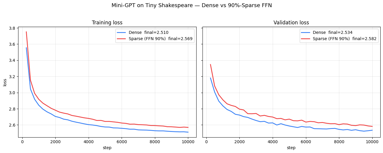
Two end-to-end results from the SparseLab v0.1 demos, measured on an M3 Pro MacBook. The transformer experiment ran three configurations side by side — dense baseline, FFN-only 90% sparse, and all-sparse (attn 70% + FFN 90%):
| Experiment | Config | Quality | Inference memory |
|---|---|---|---|
| MNIST MLP (784-512-10) | Dense | 98.06% accuracy | baseline |
| 90% sparse | 97.45% (−0.61 pp) | 82% reduction | |
| 10M Mini-GPT, Tiny Shakespeare, 10k steps | Dense | val loss 2.534 | 41.0 MB baseline |
| FFN 90% sparse | val loss 2.582 (+0.048) | 19.9 MB (48%) | |
| All sparse (attn 70% + FFN 90%) | val loss 2.589 (+0.055) | 15.3 MB (37%) |
A 0.61 pp accuracy gap on MNIST for an 82% memory reduction. A char-level transformer tracking dense val loss to within 0.055 nats even with 82% of weights removed. Here's what that tracking looks like:
We've since replicated the same pattern at 4× the scale — a 40M-parameter transformer, same architecture, same seed:
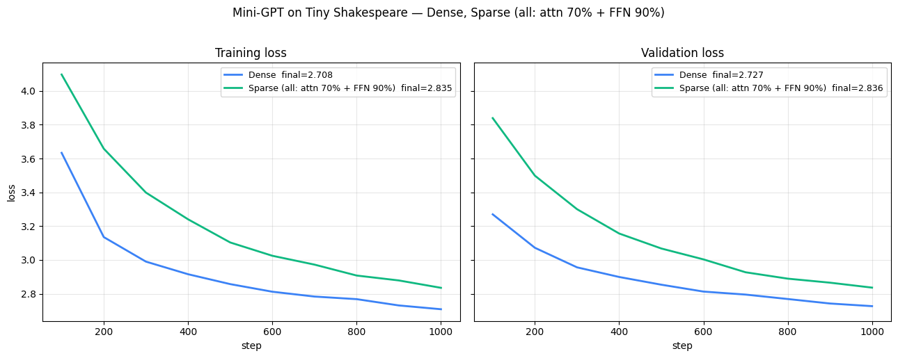
dW backward kernel isn't NEON-tuned yet (relies on Clang auto-vectorization), and sparse kernels have fixed per-layer overhead that dominates at small matrix sizes. Both are solvable. v0.2 hand-tunes dW for a ~1.3–1.5× gain, and CPU-cluster data parallelism (also v0.2) changes the scaling story entirely. Today we're honest: slower per step, meaningfully less memory, quality-preserving. The trajectory is where the argument lives.
8.2 Try It
SparseLab is MIT licensed, on PyPI, with pre-built wheels for macOS arm64 and Linux x86_64/aarch64 across Python 3.11–3.13. Install:
pip install sparselabDrop-in usage with a standard PyTorch module:
import torch
import sparselab

# One-line swap: nn.Linear → sparselab.SparseLinear
model = torch.nn.Sequential(
    sparselab.SparseLinear(784, 512, sparsity=0.9),
    torch.nn.ReLU(),
    torch.nn.Linear(512, 10),
)
opt = torch.optim.SGD(model.parameters(), lr=0.01)

# Pluggable DST: attach SET topology mutation in 2 lines.
algo = sparselab.SET(sparsity=0.9, drop_fraction=0.3, update_freq=100)
model.apply(algo)

# Rest of the training loop is plain PyTorch.
for step in range(1000):
    x = torch.randn(128, 784)
    loss = model(x).sum()
    loss.backward()
    opt.step()
    algo.step()       # drives topology mutation on the schedule
    opt.zero_grad()
SparseLinear is a standard nn.Module. Its weight is a standard nn.Parameter. It serializes through state_dict like any other layer. The only difference is what's underneath: a Padded-CSR, the SpMM kernel from Section 6, and the cached transpose from Section 7. Everything we've just walked through is in the hot path of that forward pass.
8.3 What's Next
v0.2 is focused on the scaling story:
- CPU-cluster data parallelism via PyTorch DDP. This is the one that matters. A 1B-dense-parameter model at 90% sparsity is 100M live weights — roughly 400 MB at training-time precision. That fits in RAM on any modern laptop. A 10-machine cluster with 128 GB RAM each (a few thousand dollars of commodity workstations) becomes a realistic setup for workloads that currently demand an 8×H100 DGX node.
- Hand-tuned NEON
dWkernel. The backward weight-gradient kernel is currently Clang auto-vectorized. Matching the SpMM kernel's care for memory layout and ILP should give a 1.3–1.5× end-to-end speedup at FFN scale. - AVX-512 kernels for x86. Excellent contribution target — the NEON kernel translates straightforwardly.
- Buffer reuse in the backward path. The transpose cache is one slice of this; arena-style allocators for backward temporaries is the broader version.
PaddedCSR.compact_all()primitive. For adaptive-density DST where per-row nnz changes (SET and RigL keep it fixed, so v0.1 doesn't need this).
v0.3 territory: memory-mapped weights for models that exceed node RAM, sparse attention as a first-class primitive, and a GPU backend as a community contribution target.
8.4 Contribute
Contribute. The moats are in csrc/kernels/. Every SpMM or dW optimization compounds for every user forever. If you've written hand-tuned SIMD before — NEON, AVX-512, or even RISC-V V — that's exactly the kind of contribution we want. The code is intentionally readable; a grad student should be able to open spmm_neon.cpp, understand the inner loop, and send a PR.
New DST algorithms are the other easy entry point. SET and RigL are both ~50 lines each in sparselab/router.py. Drop/grow rules from the literature (Sparse Momentum, Top-KAST, adaptive-density variants) fit the same shape.
Links
- GitHub: github.com/DarshanFofadiya/sparselab
- PyPI: pypi.org/project/sparselab
- Install:
pip install sparselab - Colab quickstart: Open in Colab
- Issues / PRs: github.com/DarshanFofadiya/sparselab/issues
If you build something with SparseLab — a new DST algorithm, a kernel port, a benchmark on hardware we haven't tested — I'd love to hear about it. Open an issue, send a PR, or email me directly.
9. What Ideal Sparse Hardware Would Look Like
SparseLab is a software stack. It runs on commodity CPUs because that's what every researcher already has. But the longer argument — the one that takes sparse from "interesting experiment" to "how AI actually gets trained" — needs hardware built for sparsity, not against it.
This section is a survey of what exists today and what would need to change. It's the most speculative section in this post; I've leaned on published sources where I can and flagged the rest as opinion.
9.1 What GPUs Do (and Don't)
Modern GPUs are dense-matmul machines that were asked to say yes to sparsity. The compromise was 2:4 structured sparsity, introduced with NVIDIA's Ampere generation and carried forward into Hopper and Blackwell. From NVIDIA's documentation: out of every four consecutive weights, exactly two must be zero, and two must be nonzero. That regularity lets the tensor cores skip half the multiplies.
2:4 STRUCTURED SPARSITY (NVIDIA Ampere+):
═════════════════════════════════════════
A row of 16 weights looks like:
  [w0 w1 w2 w3 | w4 w5 w6 w7 | w8 w9 wA wB | wC wD wE wF]
   └── 4 ──┘    └── 4 ──┘    └── 4 ──┘    └── 4 ──┘

In each group of 4, exactly 2 must be zero. The hardware
stores only the 2 live values + a 2-bit metadata that says
which positions they came from.

Best-case speedup: 2× the dense FLOP rate.
Max sparsity:      50%.
Real-world speedup: typically 1.0×–1.3× end-to-end.
The compromise is severe. Most DST algorithms converge to 80–95% sparsity, well past the 50% ceiling. Above 50%, the GPU falls back to dense matmul with zeros left in — you pay full dense cost for a sparse pattern. And empirically, one 2024 analysis of 2:4 on production workloads found real-world speedups often capped at ~1.3×, not 2×, because of memory bandwidth and scheduling overheads.
GPUs aren't designed for sparse training. NVIDIA's 2:4 tooling is inference-first: you prune a trained model, re-finetune to recover, and deploy. The topology mutations that Padded-CSR is built around — unstructured, dynamic, from-scratch sparse training — are not on the GPU roadmap.
9.2 Where Sparse Accelerators Already Exist
Some hardware does accelerate unstructured sparsity:
- Cerebras CS-2 / CS-3 (wafer-scale). Per Cerebras's documentation, their wafer-scale processor accelerates unstructured weight sparsity directly: zero weights are genuinely skipped on both forward and backward passes. This is the closest thing to "true sparse hardware" in production. The catch is that a CS-3 costs millions of dollars and is only installable in a datacenter — researchers can't experiment on one.
- Neuromorphic chips (Loihi 2, IBM NorthPole). These are brain-inspired architectures built around event-driven computation — an operation happens only when a neuron spikes, so idle neurons consume nearly zero power. Sandia's Hala Point system combines 1,152 Loihi 2 chips into a single chassis with 1.15 billion neurons. For spiking workloads, the efficiency gains are significant. The catch is that neuromorphic hardware runs spiking neural networks, which are a different computational substrate from the deep-learning models we actually want to train. Translating standard backprop-trained transformers to SNNs remains an open research problem.
- Research accelerators. Academic work like the systolic-array architectures in recent papers show that hardware co-designed for unstructured sparse matmul can hit strong efficiency numbers in simulation. Most of these designs have not shipped as silicon that researchers can buy.
The gap. Sparse accelerators exist, but either they're priced out of reach, or they target a different computational model (spiking), or they live in papers rather than fabs. The middle ground — commodity, programmable, general-purpose sparse hardware — doesn't exist yet.
9.3 What I'd Want From an Ideal Sparse Chip
This is the opinion section. Taking the concrete pain points we hit in this post and asking what hardware would make them go away:
1. Native indirect-addressed load/store at full bandwidth. The hottest operation in the SpMM kernel (Section 6.2) is "read X[col_indices[k], :] for an unpredictable col_indices[k]." On CPUs and GPUs alike, this indirect load serializes on the memory subsystem because the address isn't known until the index is fetched. An ideal sparse chip would have a gather/scatter unit designed for this pattern — so reading N non-contiguous rows of X at full bandwidth costs about what reading N contiguous rows does. AVX-512's vgather is a step in this direction but not enough; the ideal version would have dedicated address-prediction and prefetch.
2. Variable-width SIMD with compressed-index operands. Current SIMD units want dense aligned inputs. The ideal sparse SIMD instruction would take (values[], col_indices[], row_nnz) directly and produce a scaled sum into an accumulator in one instruction — the sparse equivalent of an FMA. This collapses Section 6.2's hand-written 2×-unrolled NEON loop into a single opcode.
3. Hardware-managed row capacity with O(1) insert/delete. Padded-CSR solves the mutation problem in software by reserving padding slots. A sparse-native memory subsystem could do this with hardware bookkeeping — each row is a logical free list, and inserting a live entry is a single-cycle operation that the hardware translates into an actual slot under the hood. The result: topology mutations become basically free, the 20% padding overhead disappears, and DST's dropping and growing of weights stops being something you have to budget for.
4. Transpose as a first-class primitive. The backward pass (Section 7) needs WT. On CPU we cache it. On an ideal sparse chip, both W and WT would be addressable views of the same underlying live-entry store — accessing either direction is equally fast, no copy needed. Conceptually this is a graph-storage insight (edges are both outgoing and incoming), adapted to sparse tensors.
5. Sparsity-aware memory hierarchy. At 90% sparsity, 90% of the compute is skipped but 90% of the memory bandwidth can still be wasted if the matrix is stored padded. An ideal chip would have a compressed cache line format — live values and their indices packed together, so a cache miss fetches only live data rather than padding. This is a close cousin of what GPUs did for texture compression, applied to the weight matrix itself.
6. Event-driven compute for activations. The neuromorphic angle, adapted to standard deep learning. Most ReLU activations produce zeros for most inputs. A conventional GPU multiplies past them anyway. An event-driven sparse chip would skip the downstream multiplies for any activation that fires zero — extending sparsity from “weights are sparse” to “compute follows where the signal actually flows.”
9.4 Why This Hasn't Happened Yet
The chicken-and-egg. Hardware vendors build what researchers actually run. Researchers run mask-on-dense because that's what GPUs support. Hardware vendors see dense workloads, conclude sparse is a niche, and keep investing in dense. The loop closes.
The way out is to demonstrate that actually-sparse training works, produces competitive models, and is held back by the substrate rather than the math. SparseLab's v0.1 results — a 10M-parameter transformer at 37% of dense memory, quality matching dense on a MacBook CPU — are the first data point. We've since replicated the memory story at 4× the scale (40M parameters, see Section 8.1): the 37% memory ratio holds, both paths train cleanly, and the per-step slowdown is already narrowing. If sparse training keeps working as we scale up — v0.2's CPU-cluster DDP, v0.3's memory-mapped models — then the case for building sparse silicon becomes a lot easier to make.
And then, maybe, twenty watts.
Walk away with this. Sparse neural networks are real, the lottery ticket is real, and the gap between the algorithmic case and production isn't accuracy — it's the substrate. Padded-CSR removes one piece of that gap. The rest is follow-on work on kernels, hardware, and algorithms — and with industry focus, it can move fast.
Cite this article
@misc{fofadiya2026paddedcsr,
  author       = {Darshan Fofadiya},
  title        = {Padded-CSR: A Sparse Storage Format for Dynamic Sparse Training on CPU},
  year         = {2026},
  url          = {https://darshanfofadiya.com/open-source/sparselab/}
}
Get notified when I publish new deep dives
Illustrated guides on LLM inference, quantum computing, and open-source ML.
⚠ After subscribing, check your inbox for a confirmation email. You won't receive posts until you confirm.
Comments
[email protected]